Data Drift Detector Filter Plugin¶

foglamp-filter-data-drift detects the data drift and can be a goto plugin for this application. In addition to this application this plugin can also be used to estimate the distinction or similarity between the historic or a specific signal of interest w.r.t. the current signal.

Supported Strategies & Methologies¶

This filter plugin supports five types of detection strategies and each of these strategy contains multiple methodologies. These are as following:

Distance
Here, we calculate the statistical distance between a reference signal with the current signal. The comparision helps in checking the distinction or similarity between them and generate the distance related score for the same.

This strategy is specific for 1D a.k.a. univariate signal comparision.

This strategy will only add statistic datapoint to the input assset.

This strategy supports the following measures:
- kl_divergence
  
  Kullback–Leibler Divergence (aka Relative Entropy) which tries to quantify how much one probability distribution differs from another.
- interchanged_kl_divergence
  
  Same as kl_divergence except it interchanges signal1 and signal2 so that you compare signal2 w.r.t. signal1 now.
- braycurtis
  
  Bray-Curtis checks for the dissimilarity between two samples. This results in a value between 0 and 1, where 0 indicates identical compositions and 1 indicates completely dissimilar compositions.
- canberra:
  
  Canberra distance metric is particularly useful when dealing with data containing outliers or when the relative differences between values are more important than the absolute differences.
- chebyshev
  
  Chebyshev distance is the maximum absolute difference between the corresponding components of the two vectors. It measures the greatest difference along any dimension.
- cityblock
  
  Cityblock distance is the sum of the absolute differences between the corresponding components of the two vectors. It measures the distance along axes at right angles.
- correlation
  
  Correlation is a statistical measure that describes the relationship between two variables. It indicates both the strength and direction of the relationship.
- cosine
  
  Cosine similarity measures the cosine of the angle between two vectors. If the vectors are similar, the angle between them is small, and thus the cosine similarity is close to 1. Conversely, if the vectors are dissimilar or orthogonal (at a 90-degree angle), the cosine similarity is close to 0.
- euclidean
  
  Euclidean distance is the square root of the sum of the squared differences between corresponding coordinates of the two points.
- jensenshannon
  
  JS Divergence uses the KL divergence. The main differences between JS divergence and KL divergence are that JS is symmetric and it always has a finite value. It is Versatile in nature. It doesn’t differentiate between very strong and extreme drifts. Range [0,1]
- minkowski
- sqeuclidean
  
  Compared to the Euclidean distance, which involves taking the square root of this sum, the squared Euclidean distance does not involve the square root operation. This means that it’s computationally cheaper to compute and can be used when the actual distance values are not needed.
- wasserstein
  
  Wasserstein Distance is sensitive to outlier and is recommeded to be used where a shift in measure is relevant. Range [0,inf).
- energy
  
  Energy distance is used to quantify the discrepancy between two probability distributions. It provides a way to compare the closeness of two distributions in a nonparametric manner.
- l_infinity
  
  L-Infinity is sensitive to big changes to one category. This measure is not to be used with continous data.
- psi
  
  Population Stability Index is used to measure how much the distribution of a variable has changed between two samples or over time. A high PSI value indicates that there is a significant difference between the distributions of the variable in the two datasets, which may suggest that there is a drift in the model.
  
  When
  - PSI<0.1; means very low change between the two groups, considered stable.
  - 0.1<= PSI<0.25; means moderate change between the two groups.
  - PSI>=0.25; means significant change.
Independance test
Here, we calculate the statistical independance between these two signal namely a reference signal with the current signal. The comparision helps in checking the distinction or similarity between them and generate the distance related score for the same.

This strategy is specific for 1D a.k.a. univariate signal comparision.

This strategy will add statistic and pvalue datapoint to the input assset. Though with the ks_2samp methodology this will additionally create statistic_location and statistic_sign datapoints too.

This strategy supports the following measures:
- ttest_ind
  
  Independent samples t-test, can be used to determine if there is a significant difference between the means of two independent groups.
- mannwhitneyu
  
  Mann-Whitney U test, also known as the Wilcoxon rank-sum test, is a nonparametric statistical test used to determine whether two independent samples come from populations having the same distribution. It’s commonly used as an alternative to the independent samples t-test when the assumptions of normality and equal variances are not met, or when the data is ordinal or not normally distributed.
- ranksums
  
  Perform the Wilcoxon rank-sum test, which is equivalent to the Mann-Whitney U test. This function allows you to compare the means of two independent samples to determine whether they come from the same distribution, without assuming normality of the data.
- brunnermunzel
  
  Brunner-Munzel test is a nonparametric statistical test used to compare the distributions of two independent samples. It’s particularly useful when the assumptions of normality and homogeneity of variances are not met.
- mood
  
  Mood’s median test is a nonparametric statistical test used to determine whether two or more independent samples have the same population median. It’s a useful test when the assumptions of parametric tests, such as the t-test or analysis of variance (ANOVA), are not met, particularly when dealing with ordinal or skewed data.
- ansari
  
  Ansari-Bradley test, also known simply as the Ansari test, is a nonparametric statistical test used to compare the distributions of two independent samples in terms of their medians. It’s similar to the Mann-Whitney U test but uses a different test statistic.
- cramervonmises_2samp
  
  Cramer-von Mises two-sample test is a statistical test used to compare the distributions of two independent samples. It’s a nonparametric test and is particularly useful when the assumptions of parametric tests are not met or when dealing with ordinal or skewed data.
- epps_singleton_2samp
  
  Epps-Singleton two-sample test is a nonparametric statistical test used to compare the distributions of two independent samples. It’s particularly useful when the assumptions of parametric tests, such as normality or equal variances, are not met.
- ks_2samp
  
  The Kolmogorov-Smirnov two-sample test (KS test) is a nonparametric statistical test used to compare two independent samples to determine if they are drawn from the same underlying probability distribution. It’s particularly useful when comparing samples with unknown distributions or when the data is not normally distributed.
Distribution test
Here, the recently collected readings are used for distribution calculation and the samples are compared with some generally known distribution to see how closer we are to the mentioned distribution.

This strategy is specific for 1D a.k.a. univariate signal comparision.

This strategy will add statistic, pvalue, statistic_location and statistic_sign datapoint to the input assset.

This strategy supports the following measures:
- norm
  
  Normal distribution aka Gaussian distribution is characterized by a bell-shaped curve when plotted as a probability density function. The normal distribution is symmetric around its mean, and its shape is determined by the mean and variance. The mean represents the center of the distribution, while the variance controls the spread or dispersion of the distribution.
- uniform
  
  The uniform distribution is a probability distribution where all outcomes within a specified range are equally likely. It’s characterized by a constant probability density function (PDF) within its range. The uniform distribution is symmetric and flat within its range. Every value within the range has the same probability of occurring. Outside the range, the PDF is zero.
- cosine
  
  The cosine distribution, is a continuous probability distribution on the unit circle in the plane. It’s commonly used to model directional data or angular data that is symmetrically distributed around a central angle.
- expon
  
  The exponential distribution is a continuous probability distribution that models the time between events in a Poisson process, where events occur continuously and independently at a constant rate over time.
- arcsine
  
  The arcsine distribution, also known as the “inverse sine” distribution, is a continuous probability distribution on the interval [a,b] where 0<=a<b<=1. It is often used to model probabilities or random variables that are constrained to lie within a certain range, such as probabilities or angles. The arcsine distribution has a U-shaped PDF, with higher density near the endpoints a and b, and lower density in the middle. It is symmetric around the midpoint (a+b)/2.
- cauchy
  
  The Cauchy distribution, is a continuous probability distribution that is notable for its heavy tails and lack of finite moments (except for the first moment, which is undefined if the distribution is symmetric).
- anglit
- gibrat
- gumbel_r
- gumbel_l
- halfcauchy
- halflogistic
- halfnorm
- hypsecant
- kstwobign
- laplace
- levy
- levy_l
- logistic
- maxwell
- moyal
- rayleigh
- semicircular
- wald
Process Control
The idea of statistical process control is to verify that our model’s error is in control. This is especially important when running in production as the performance changes over time. Thus, we would like to have a system that would send an alert if the model passes some error rate. Note that some models have a “traffic light” system where they also have warning alerts.

This strategy is specific for 1D a.k.a. univariate signal comparision.

This strategy will only add statistic datapoint to the input assset.

This strategy supports the following measures:
- adwin
  
  ADaptive WINdowing is an adaptive sliding window algorithm for detecting change, and keeping updated statistics about a data stream. ADWIN allows algorithms not adapted for drifting data, to be resistant to this phenomenon. Default Parameters: {'delta':0.002}
- ddm
  
  Drift Detection Method is a concept change detection method based on the PAC learning model premise, that the learner’s error rate will decrease as the number of analysed samples increase, as long as the data distribution is stationary. Default Parameters: {"min_num_instances": 30, "warning_level": 2.0, "out_control_level": 3.0}
- eddm
  
  EDDM (Early Drift Detection Method) aims to improve the detection rate of gradual concept drift in DDM, while keeping a good performance against abrupt concept drift. This method works by keeping track of the average distance between two errors instead of only the error rate. For this, it is necessary to keep track of the running average distance and the running standard deviation, as well as the maximum distance and the maximum standard deviation. Default Parameters: {}
- hddm_a
  
  HDDM_A is a drift detection method based on the Hoeffding’s inequality. HDDM_A uses the average as estimator. Default Parameters: {"drift_confidence": 0.001, "warning_confidence": 0.005, "two_side_option": True}
- hddm_w
  
  HDDM_W is an online drift detection method based on McDiarmid’s bounds. HDDM_W uses the EWMA statistic as estimator. Default Parameters: {"drift_confidence": 0.001, "warning_confidence": 0.005, "lambda_option": 0.05, "two_side_option": True}
- kswin
  
  KSWIN (Kolmogorov-Smirnov Windowing) is a concept change detection method based on the Kolmogorov-Smirnov (KS) statistical test. KS-test is a statistical test with no assumption of underlying data distribution. KSWIN can monitor data or performance distributions. Default Parameters: {"alpha": 0.005, "window_size": 100, "stat_size": 30, "data": None}
- page_hinkley
  
  The Page-Hinkley algorithm, also known as the Page’s Cumulative Sum (CUSUM) algorithm, a statistical method used for monitoring changes or shifts in a sequence of data over time. It’s particularly useful for detecting abrupt changes or anomalies in time series data. The Page-Hinkley algorithm is useful for detecting both abrupt changes (e.g., sudden shifts in mean or variance) and gradual changes (e.g., trends or drifts) in time series data. Default Parameters: {"min_instances": 30, "delta": 0.005, "threshold": 50, "alpha": 0.9999}
Multivariate PCA Reconstruction
This method is able to capture complex changes in our data. As PCA will learn the internal structure of the data, a significant change in the reconstruction error means that the learned structure no longer accurately approximates the current data structure. This indicates data drift.

To detect the drift that can’t be seen on 1D data we can use this strategy. This can be used with multi dimensional data a.k.a. multivariate signal comparision.

This strategy will add statistic and std datapoint to the input assset.

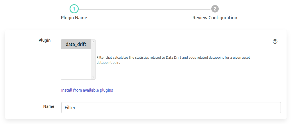
Plugin Configurations¶

Configuring filter, starts with selecting the filter and adding a service name for it. The screen will look like the following.

screen_plugin_selection

Following this the configurations are grouped under 6 sections. Namely,

Inputs : This will deal with selecting the input time series data.
Strategy : Decide on how to detect data drift.
Output-Statistic : Decide the output datapoint name which will hold the statistics value.
Output-Warning : Decide on when to raise the warning and how to add the datapoint.
Output-Alert : Decide on when to raise the alert and how to add the datapoint.
Trigger Interval : Decide on when to perform the detection.

Inputs¶

screen_inputs

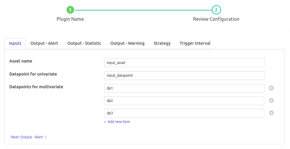
‘Asset name’: type: `string` default: ‘input_asset’:
Asset name of the data that will be the input to filter.
‘Datapoint for univariate’: type: `string` default: ‘input_datapoint’:
Asset attribute (datapoint) which will be the input to filter. Note: This must have numeric data.
‘Datapoint for multivariate’: type: `list` default: ‘[“dp1”,”dp2”,”dp3”]’:
Datapoints to be used for drift detection in Multivariate. Note: use this when 2 or more datapoints are to be used.

Strategy¶

screen_strategy

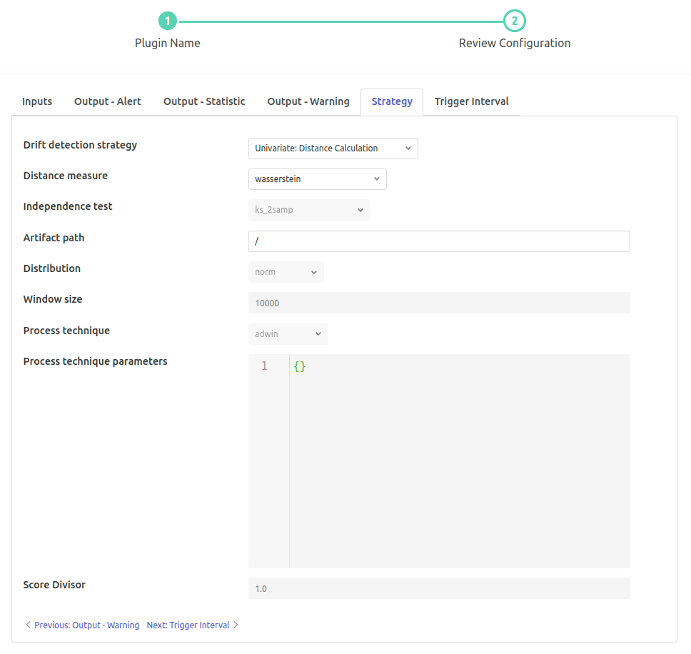
‘Drift detection strategy’: type: `enumeration` default: ‘Univariate: Distance Calculation’:

Select a Data Drift Detection Strategy. Options
- Univariate: Distance Calculation
- Univariate: Independence Tests
- Univariate: Distribution Comparision
- Univariate: Process Control
- Multivariate: PCA Reconstruction
‘Distance measure’: type: `enumeration` default: ‘Simple (Non-Weighted)’:

The measure that is to be used for distance calculation. Options
- kl_divergence
- interchanged_kl_divergence
- braycurtis
- canberra
- chebyshev
- cityblock
- correlation
- cosine
- euclidean
- jensenshannon
- minkowski
- sqeuclidean
- wasserstein
- energy
- l_infinity
- psi
‘Independence test’: type: `enumeration` default: ‘Simple (Non-Weighted)’:

The test which is to be used for calculating the Independence. Options
- ttest_ind
- mannwhitneyu
- ranksums
- brunnermunzel
- mood
- ansari
- cramervonmises_2samp
- epps_singleton_2samp
- ks_2samp
‘Artifact path’: type: `string` default: ‘/’:

Add abs path in here. Path to the .npy artifact containing a 1D sequence or pkl artifact containing the pca pipeline model.
‘Distribution’: type: `enumeration` default: ‘norm’:

Distribution which is be used for comparison Options
- norm
- uniform
- anglit
- arcsine
- cauchy
- cosine
- expon
- gibrat
- gumbel_r
- gumbel_l
- halfcauchy
- halflogistic
- halfnorm
- hypsecant
- kstwobign
- laplace
- levy
- levy_l
- logistic
- maxwell
- moyal
- norm
- rayleigh
- semicircular
- wald
‘Window size’: type: `integer` default: ‘10000’:

Sequence Length i.e. to be used for the samples to check distribution calculation.
‘Process technique’: type: `enumeration` default: ‘adwin’:

Process Control Techique Options
- adwin
- ddm
- eddm
- hddm_a
- hddm_w
- kswin
- page_hinkley
‘Process technique parameters’: type: `JSON` default: ‘{}’:

Accept dictionary containing the params for the technique selected under Process Technique.
‘Score Divisor’: type: `float` default: ‘1.0’:

Provide a value if you want the statistics to be divided by this number to convert it to ratio.

Output-Statistic¶

screen_output_statistic

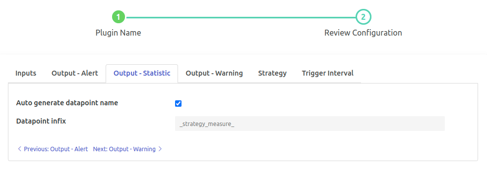
‘Auto generate datapoint name’: type: `boolean` default: ‘true’:

Automatically decide the Output datapoint name based on selected measures {{Input Datapoint}}{{Infix}}{{Suffix}} 2nd part will be added.
‘Datapoint infix’: type: `string` default: ‘_strategy_measure_’:

Output datapoint name will follow the pattern {{Input Datapoint}}{{Infix}}{{Suffix}} 2nd part is customizable.

Output-Warning¶

screen_output_warning

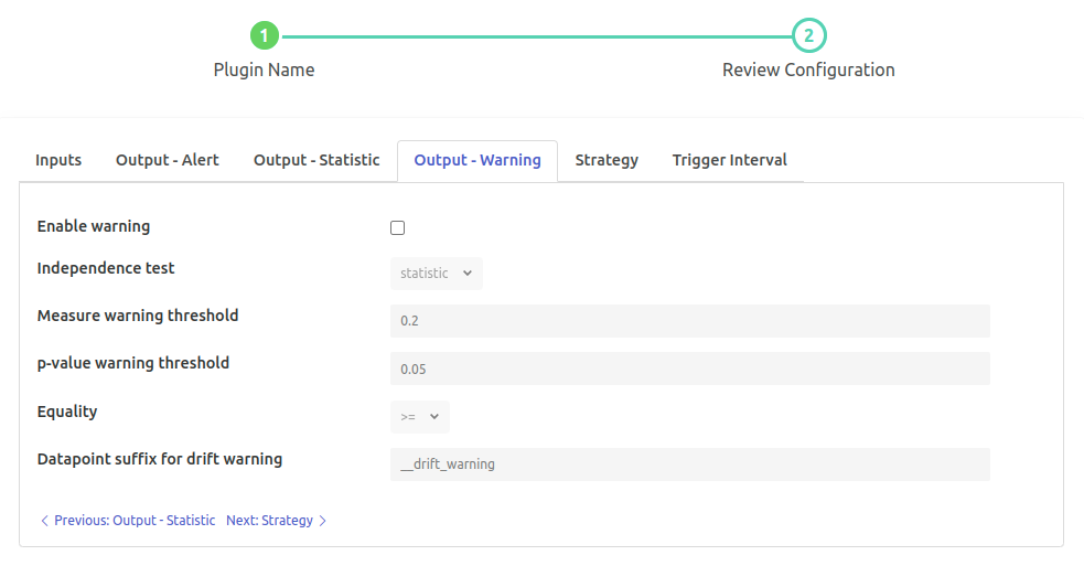
‘Enable warning’: `boolean` default: ‘false’:

Enable warning for data drift
‘Independence test’: `enumeration` default: ‘statistic’:

The test which is to be used for calculating the Independence. ‘pvalue’ is not supported with ‘distance’ strategy. Options
- statistic
- pvalue
‘Measure warning threshold’: type: `float` default: ‘0.2’:

Statistic value that will be used for threshold. In case drift score exceeds/subceed this score, True (1) will be added to data drift warning datapoint.
‘p-value warning threshold’: type: `float` default: ‘0.05’:

p-value that will be used for threshold. Note: If greyed then this is not supported for the algorithm. In case drift score exceeds/subceed this score, True (1) will be added to data drift warning datapoint.
‘Equality’: type: `enumeration` default: ‘>=’:

Raise the warning w.r.t. the equality and score Options
- >
- >=
- <
- <=
‘Datapoint suffix for drift warning’: type: `string` default: ‘__drift_warning’:

Suffix for the output datapoint name for warning wrt drift. Output datapoint name will have the pattern “{{Input Datapoint}}{{Suffix }}” 2nd part is customizable.

Output-Alert¶

screen_output_alert

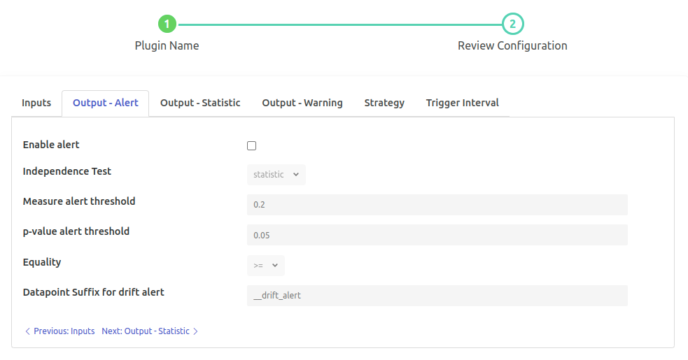
‘Enable alert’: `boolean` default: ‘false’:

Enable alert for data drift
‘Independence test’: `enumeration` default: ‘statistic’:

The test which is to be used for calculating the Independence. ‘pvalue’ is not supported with ‘distance’ strategy. Options
- statistic
- pvalue
‘Measure alert threshold’: type: `float` default: ‘0.2’:

Statistic value that will be used for threshold. In case drift score exceeds/subceed this score, True (1) will be added to data drift alert datapoint.
‘p-value alert threshold’: type: `float` default: ‘0.05’:

p-value that will be used for threshold. . Note: If greyed then this is not supported for the algorithm. In case drift score exceeds/subceed this score, True (1) will be added to data drift alert datapoint.
‘Equality’: type: `enumeration` default: ‘>=’:

Raise the alert w.r.t. the equality and score Options
- >
- >=
- <
- <=
‘Datapoint suffix for drift alert’: type: `string` default: ‘__drift_alert’:

Suffix for the output datapoint name for alert wrt drift. Output datapoint name will have the pattern {{Input Datapoint}}{{Suffix }} 2nd part is customizable.

Trigger Interval¶

screen_trigger_interval

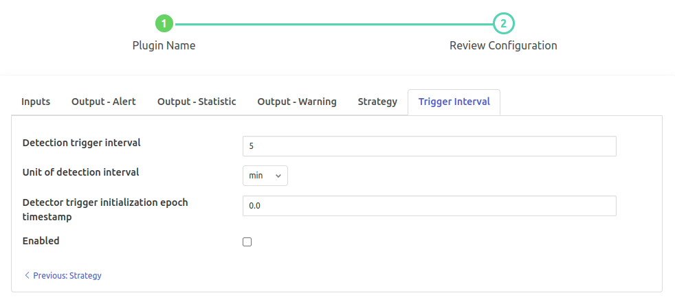
Detection trigger Interval’: type: `float` default: ‘5’:

approximately it will be wrt to the initialization time.
‘Unit of Detection Interval’: `enumeration` default: ‘min’:

Time interval units Options
- sec
- min
- hour
- day
‘Detector trigger initialization epoch timestamp’: type: `float` default: ‘0.0’:

Initialization epoch timestamp for the trigger detection. Note: execution will start from the next iteration from this timestamp.
‘Enabled’: `boolean` default: ‘false’:

Enable Data Drift Detection filter plugin

Click on Done when ready.